CytoSimplex.plot_quaternary

CytoSimplex.plot_quaternary(x, cluster_var, vertices, features=None, velo_graph=None, save_fig=False, fig_path='plot_quaternary.png', fig_size=None, processed=False, method='euclidean', force=False, sigma=0.05, scale=True, title=None, split_cluster=False, cluster_title=True, dot_color='#8E8E8EFF', n_velogrid=10, radius=0.16, elev=5, azim=10, roll=0, dot_size=0.6, vertex_colors=['#3B4992FF', '#EE0000FF', '#008B45FF', '#631879FF'], vertex_label_size=12, arrow_linewidth=1.0)

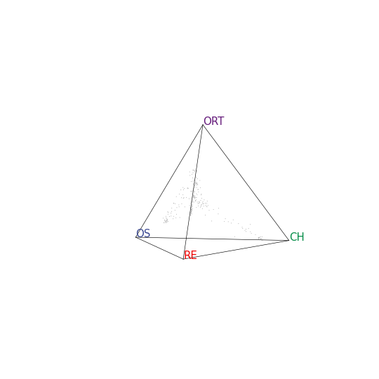
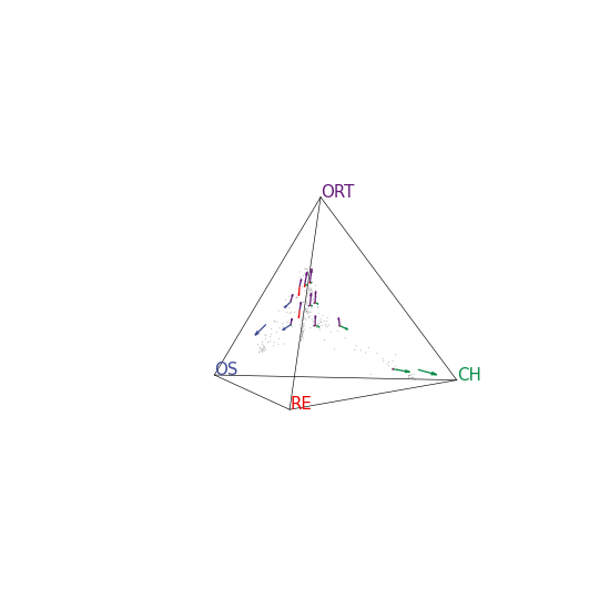
Create ternary plot that shows the similarity between each single cell and the four vertices of a simplex (tetrahedron) which represents specified clusters. Velocity information can be added to the plot. The view angle of the plot can be adjusted via elev, azim and roll. When in an interactive session, the plot shown in pop-out window is interactive. If an interactive view is desired, Jupyter Notebook users will need to have package “ipympl” pre-installed and add the line %matplotlib widget at the top of the code block.

Parameters

• x (Union[AnnData, ndarray, csr_matrix]) – Object that has the expression matrix of the single cells. Each row represents a single cell and each column represents a gene.

• cluster_var (Union[str, list, Series]) – The cluster assignment of each single cell. If x is an anndata.AnnData, cluster_var can be a str that specifies the name of the cluster variable in x.obs. list or pandas.Series is accepted in all cases, and the length must equal to x.shape[0].

• vertices (Union[list, dict]) –

  The terminal specifications. Should have exactly 4 elements for the 3-simplex (quaternary simplex / tetrahedron). Acceptable input include:

  • A list of 4 str that exist in the categories of cluster_var.

  • A dict of 4 keys. The keys are presented as customizable vertex names. The corresponding value for each key can be either a str for a single cluster, or a list of str for grouped vertex of multiple clusters.

• features (Optional[list[str]]) – The features to be used in the calculation of similarity. It is recommended to derive this list with select_top_features(). Default uses all features.

• velo_graph (Union[csr_matrix, str, None]) – The velocity graph of the single cells, presented as an n-by-n sparse matrix. When x is anndata.AnnData, velo_graph can be a str to be used as a key to retrieve the appropiate data from x.uns. By default, no velocity information will be added to the plot.

• save_fig (bool) – Whether to save the figure.

• fig_path (str) – The path to save the figure.

• fig_size (Optional[Tuple[int, int]]) – The size of the figure. The first number for width and the second for height.

• processed (bool) – Whether the input matrix is already processed. When False, a raw count matrix (with integers) is recommended and preprocessing of library-size normalization, scaled log1p transformation will happen internally. If True, the input matrix will directly be used for computing the similarity.

• method (str) – Choose from “euclidean”, “cosine”, “pearson” and “spearman”. When “euclidean” or “cosine”, the similarity is converted from the distance with a Gaussian kernel and the argument sigma would be applied. When “pearson” or “spearman”, the similarity is derived as the correlation is.

• force (bool) – Whether to force the calculation when the number of features exceeds 500.

• sigma (float) – The sigma parameter in the Gaussian kernel that converts the distance metrics into similarity.

• scale (bool) – Whether to scale the similarity matrix by vertices.

• title (Optional[str]) – The title of the plot. Not used when split_cluster=True.

• split_cluster (bool) – Whether to split the plot by clusters. If False, all cells will be plotted in one plot. If True, the cells will be split by clusters and each cluster will be plotted in one subplot.

• cluster_title (bool) – Whether to show the cluster name as the title of each subplot when split_cluster=True.

• dot_color (str) – The color of the dots.

• n_velogrid (int) – The number of square grids, along the bottom side of the triangle, to aggregate the velocity of cells falling into each grid.

• radius (float) – Scaling factor of aggregated velocity to get the arrow length.

• elev (float) – The elevation angle in the z plane.

• azim (float) – The azimuth angle in the x,y plane.

• roll (float) – The roll angle in the x,y plane.

• dot_size (float) – The size of the dots.

• vertex_colors (list[str, str, str, str]) – The colors of the vertex labels, grid lines, axis labels and arrows.

• vertex_label_size (int) – The size of the vertex labels.

• arrow_linewidth (float) – The linewidth of the arrows.

Return type

Figure will be shown or saved.

Examples

The 3-simplex (i.e. simplex in 3D, which is a tetrahedron) visualized by Matplotlib is indeed interactive in users interactive session.

import CytoSimplex as csx
import scanpy as sc
adata = sc.read(
    filename="test.h5ad",
    backup_url="https://figshare.com/ndownloader/files/41034857"
)
vertices = {'OS': ["Osteoblast_1", "Osteoblast_2", "Osteoblast_3"],
            'RE': ['Reticular_1', 'Reticular_2'],
            'CH': ['Chondrocyte_1', 'Chondrocyte_2', 'Chondrocyte_3'],
            'ORT': ['ORT_1', 'ORT_2']}
gene = csx.select_top_features(adata, "cluster", vertices)
csx.plot_quaternary(adata, "cluster", vertices, gene)
csx.plot_quaternary(adata, "cluster", vertices, gene, velo_graph='velo')